Tag Archives: Broken Symmetries

Jahn-Teller Distortion and Symmetry Breaking

The Jahn-Teller effect occurs in molecular systems, as well as solid state systems, where a molecular complex distorts, resulting in a lower symmetry. As a consequence, the energy of certain occupied molecular states is reduced. Let me first describe the phenomenon before giving you a little cartoon of the effect.

First, consider, just as an example, a manganese atom with valence 3d^4, surrounded by an octahedral cage of oxygen atoms like so (image taken from this thesis):

Jahn-Teller.png

The electrons are arranged such that the lower triplet of orbital states each contain a single “up-spin”, while the higher doublet of orbitals only contains a single “up-spin”, as shown on the image to the left. This scenario is ripe for a Jahn-Teller distortion, because the electronic energy can be lowered by splitting both the doublet and the triplet as shown on the image on the right.

There is a very simple, but quite elegant problem one can solve to describe this phenomenon at a cartoon level. This is the problem of a two-dimensional square well with adjustable walls. By solving the Schrodinger equation, it is known that the energy of the two-dimensional infinite well has solutions of the form:

E_{i,j} = \frac{h}{8m}(i^2/a^2 + j^2/b^2)                where i,j are integers.

Here, a and b denote the lengths of the sides of the 2D well. Since it is only the quantity in the brackets that determine the energy levels, let me factor out a factor of \gamma = a/b and write the energy dependence in the following way:

E \sim i^2/\gamma + \gamma j^2

Note that \gamma is effectively an anisotropy parameter, giving a measure of the “squareness of the well”. Now, let’s consider filling up the levels with spinless electrons that obey the Pauli principle. These electrons will fill up in a “one-per-level” fashion in accordance with the fermionic statistics. We can therefore write the total energy of the N-fermion problem as so:

E_{tot} \sim \alpha^2/ \gamma + \gamma \beta^2

where \alpha and \beta parameterize the energy levels of the N electrons.

Now, all of this has been pretty simple so far, and all that’s really been done is to re-write the 2D well problem in a different way. However, let’s just systematically look at what happens when we fill up the levels. At first, we fill up the E_{1,1} level, where \alpha^2 = \beta^2 = 1^2. In this case, if we take the derivative of E_{1,1} with respect to \gamma, we get that \gamma_{min} = 1 and the well is a square.

For two electrons, however, the well is no longer a square! The next electron will fill up the E_{2,1} level and the total energy will therefore be:

E_{tot} \sim 1/\gamma (1+4) + \gamma (1+1),

which gives a \gamma_{min} = \sqrt{5/2}!

Why did this breaking of square symmetry occur? In fact, this is very closely related to the Jahn-Teller effect. Since the level is two-fold degenerate (i.e. E_{2,1} =  E_{1,2}), it is favorable for the 2D well to distort to lower its electronic energy.

Notice that when we add the third electron, we get that:

E_{tot} \sim 1/\gamma (1+4+1) + \gamma (1+1+4)

and \gamma_{min} = 1 again, and we return to the system with square symmetry! This is also quite similar to the Jahn-Teller problem, where, when all the states of the degenerate levels are filled up, there is no longer an energy to be gained from the symmetry-broken geometry.

This analogy is made more complete when looking at the following level scheme for different d-electron valence configurations, shown below (image taken from here).

highSpin_Jahnteller

The black configurations are Jahn-Teller active (i.e. prone to distortions of the oxygen octahedra), while the red are not.

In condensed matter physics, we usually think about spontaneous symmetry breaking in the context of the thermodynamic limit. What saves us here, though, is that the well will actually oscillate between the two rectangular configurations (i.e. horizontal vs. vertical), preserving the original symmetry! This is analogous to the case of the ammonia (NH_3) molecule I discussed in this post.

Landau Theory and the Ginzburg Criterion

The Landau theory of second order phase transitions has probably been one of the most influential theories in all of condensed matter. It classifies phases by defining an order parameter — something that shows up only below the transition temperature, such as the magnetization in a paramagnetic to ferromagnetic phase transition. Landau theory has framed the way physicists think about equilibrium phases of matter, i.e. in terms of broken symmetries. Much current research is focused on transitions to phases of matter that possess a topological index, and a major research question is how to think about these phases which exist outside the Landau paradigm.

Despite its far-reaching influence, Landau theory actually doesn’t work quantitatively in most cases near a continuous phase transition. By this, I mean that it fails to predict the correct critical exponents. This is because Landau theory implicitly assumes that all the particles interact in some kind of average way and does not adequately take into account the fluctuations near a phase transition. Quite amazingly, Landau theory itself predicts that it is going to fail near a phase transition in many situations!

Let me give an example of its failure before discussing how it predicts its own demise. Landau theory predicts that the specific heat should exhibit a discontinuity like so at a phase transition:

specificheatlandau

However, if one examines the specific heat anomaly in liquid helium-4, for example, it looks more like a divergence as seen below:

lambda_transition

So it clearly doesn’t predict the right critical exponent in that case. The Ginzburg criterion tells us how close to the transition temperature Landau theory will fail. The Ginzburg argument essentially goes like so: since Landau theory neglects fluctuations, we can see how accurate Landau theory is going to be by calculating the ratio of the fluctuations to the order parameter:

E_R = |G(R)|/\eta^2

where E_R is the error in Landau theory, |G(R)| quantifies the fluctuations and \eta is the order parameter. Basically, if the error is small, i.e. E_R << 1, then Landau theory will work. However, if it approaches \sim 1, Landau theory begins to fail. One can actually calculate both the order parameter and the fluctuation region (quantified by the two-point correlation function) within Landau theory itself and therefore use Landau theory to calculate whether or not it will fail.

If one does carry out the calculation, one gets that Landau theory will work when:

t^{(4-d)/2} >> k_B/\Delta C \xi(1)^d  \equiv t_{L}^{(4-d)/2}

where t is the reduced temperature, d is the dimension, \xi(1) is the dimensionless mean-field correlation length at T = 2T_C (extrapolated from Landau theory) and \Delta C/k_B is the change in specific heat in units of k_B, which is usually one per degree of freedom. In words, the formula essentially counts the number of degrees of freedom in a volume defined by  \xi(1)^d. If the number of degrees of freedom is large, then Landau theory, which averages the interactions from many particles, works well.

So that was a little bit of a mouthful, but the important thing is that these quantities can be estimated quite well for many phases of matter. For instance, in liquid helium-4, the particle interactions are very short-ranged because the helium atom is closed-shell (this is what enables helium to remain a liquid all the way down to zero temperatures at ambient conditions in the first place). Therefore, we can assume that \xi(1) \sim 1\textrm{\AA}, and hence t_L \sim 1 and deviations from Landau theory can be easily observed in experiment close to the transition temperature.

Despite the qualitative similarities between superfluid helium-4 and superconductivity, a topic I have addressed in the past, Landau theory works much better for superconductors. We can also use the Ginzburg criterion in this case to calculate how close to the transition temperature one has to be in order to observe deviations from Landau theory. In fact, the question as to why Ginzburg-Landau theory works so well for BCS superconductors is what awakened me to these issues in the first place. Anyway, we assume that \xi(1) is on the order of the Cooper pair size, which for BCS superconductors is on the order of 1000 \textrm{\AA}. There are about 10^8 particles in this volume and correspondingly, t_L \sim 10^{-16} and Landau theory fails so close to the transition temperature that this region is inaccessible to experiment. Landau theory is therefore considered to work well in this case.

For high-Tc superconductors, the Cooper pair size is of order 10\textrm{\AA} and therefore deviations from Landau theory can be observed in experiment. The last thing to note about these formulas and approximations is that two parameters determine whether Landau theory works in practice: the number of dimensions and the range of interactions.

*Much of this post has been unabashedly pilfered from N. Goldenfeld’s book Lectures on Phase Transitions and the Renormalization Group, which I heartily recommend for further discussion of these topics.

Broken Symmetry and Degeneracy

Often times, when I understand a basic concept I had struggled to understand for a long time, I wonder, “Why in the world couldn’t someone have just said that?!” A while later, I will then return to a textbook or paper that actually says precisely what I wanted to hear. I will then realize that the concept just wouldn’t “stick” in my head and required some time of personal and thoughtful deliberation. It reminds me of a humorous quote by E. Rutherford:

All of physics is either impossible or trivial.  It is impossible until you understand it and then it becomes trivial.

I definitely experienced this when first studying the relationship between broken symmetry and degeneracy. As I usually do on this blog, I hope to illustrate the central points within a pretty rigorous, but mostly picture-based framework.

For the rest of this post, I’m going to follow P. W. Anderson’s article More is Different, where I think these ideas are best addressed without any equations. However, I’ll be adding a few details which I wished I had understood upon my first reading.

If you Google “ammonia molecule” and look at the images, you’ll get something that looks like this:

ammonia

With the constraint that the nitrogen atom must sit on a line through the center formed by the triangular network of hydrogen atoms, we can approximate the potential to be one-dimensional. The potential along the line going through the center of the hydrogen triangle will look, in some crude approximation, something like this:

AmmoniaPotential

Notice that the molecule has inversion (or parity) symmetry about the triangular hydrogen atom network. For non-degenerate wavefunctions, the quantum stationary states must also be parity eigenstates. We expect, therefore, that the stationary states will look something like this for the ground state and first excited state respectively:

SymmetricDoubleWell

Ground State

AntiSymmetricDoubleWell

First Excited State

The tetrahedral (pyramid-shaped) ammonia molecule in the image above is clearly not inversion symmetric, though. What does this mean? Well, it implies that the ammonia molecule in the image above cannot be an energy eigenstate. What has to happen, therefore, is that the ammonia molecule has to oscillate between the two configurations pictured below:

ammoniaInversion

The oscillation between the two states can be thought of as the nitrogen atom tunneling from one valley to the other in the potential energy diagram above. The oscillation occurs about 24 billion times per second or with a frequency of 24 GHz.

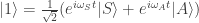
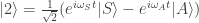
To those familiar with quantum mechanics, this is a classic two-state problem and there’s nothing particularly new here. Indeed, the tetrahedral structures can be written as linear combinations of the symmetric and anti-symmetric states as so:

| 1 \rangle = \frac{1}{\sqrt{2}} (e^{i \omega_S t}|S\rangle +e^{i \omega_A t}|A\rangle)

| 2 \rangle = \frac{1}{\sqrt{2}} (e^{i \omega_S t}|S\rangle -e^{i \omega_A t}|A\rangle)

One can see that an oscillation frequency of \omega_S-\omega_A will result from the interference between the symmetric and anti-symmetric states.

The interest in this problem, though, comes from examining a certain limit. First, consider what happens when one replaces the nitrogen atom with a phosphorus atom (PH3): the oscillation frequency decreases to about 0.14 MHz, about 200,000 times slower than NH3. If one were to do the same replacement with an arsenic atom instead (AsH3), the oscillation frequency slows down to 160 microHz, which is equivalent to about an oscillation every two years!

This slowing down can be simply modeled in the picture above by imagining the raising of the barrier height between the two valleys like so:

HighBarrierPotential

In the case of an amino acid or a sugar, which are both known to be chiral, the period of oscillation is thought to be greater than the age of the universe. Basically, the molecules never invert!

So what is happening here? Don’t worry, we aren’t violating any laws of quantum mechanics.

As the barrier height reaches infinity, the states in the well become degenerate. This degeneracy is key, because for degenerate states, the stationary states no longer have to be inversion-symmetric. Graphically, we can illustrate this as so:

SymmetricDegenerate

Symmetric state, E=E_0

Anti-symmetricDegenerate

Anti-symmetric state, E=E_0

We can now write for the symmetric and anti-symmetric states:

| 1 \rangle = e^{i\omega t} \frac{1}{\sqrt{2}} (|S\rangle + |A\rangle)

| 2 \rangle = e^{i\omega t} \frac{1}{\sqrt{2}} (|S\rangle - |A\rangle)

These are now bona-fide stationary states. There is therefore a deep connection between degeneracy and the broken symmetry of a ground state, as this example so elegantly demonstrates.

When there is a degeneracy, the ground state no longer has to obey the symmetry of the Hamiltonian.

Technically, the barrier height never reaches infinity and there is never true degeneracy unless the number of particles in the problem (or the mass of the nitrogen atom) approaches infinity, but let’s leave that story for another day.
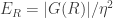
Macroscopic Wavefunctions, Off-Diagonal Long Range Order and U(1) Symmetry Breaking

Steven Weinberg wrote a piece a while ago entitled Superconductivity for Particular Theorists (pdf!). Although I have to admit that I have not followed the entire mathematical treatment in this document, I much appreciate the conceptual approach he takes in asking the following question:

How can one possibly use such approximations (BCS theory and Ginzburg-Landau theory) to derive predictions about superconducting phenomena that are essentially of unlimited accuracy?

He answers the question by stating that the general features of superconductivity can be explained using the fact that there is a spontaneous breakdown of electromagnetic gauge invariance. The general features he demonstrates are due to broken gauge invariance are the following:

  1. The Meissner Effect
  2. Flux Quantization
  3. Infinite Conductivity
  4. The AC Josephson Effect
  5. Vortex Lines

Although not related to this post per se, he also makes the following (somewhat controversial) comment that I have to admit I am quoting a little out of context:

“…superconductivity is not macroscopic quantum mechanics; it is the classical field theory of  a Nambu-Goldstone field”

Now, while it may be true that one can derive the phenomena in the list above using the formalism outlined by Weinberg, I do think that there are other ways to obtain similar results that may be just as general. One way to do this is to assume the existence of a macroscopic wave function. This method is outlined in this (illuminatingly simple) set of lecture notes by M. Beasley (pdf!).

Another general formalism is outlined by C.N. Yang in this RMP, where he defines the concept of off-diagonal long range order for a tw0-particle density matrix. ODLRO can be defined for a single-particle density matrix in the following way:

\lim_{|r-r'| \to \infty} \rho(r,r') \neq 0

This can be easily extended to the case of a two-particle density matrix appropriate for Cooper pairing (see Yang).

Lastly, there is a formalism similar to that of Yang’s as outlined by Leggett in his book Quantum Liquids, which was first developed by Penrose and Onsager. They conclude that many properties of Bose-Einstein Condensation can be obtained from again examining the diagonalized density matrix:

\rho(\textbf{r},\textbf{r}';t) = \sum_i n_i(t)\chi_i^*(\textbf{r},t)\chi_i(\textbf{r}',t)

Leggett then goes onto say

“If there is exactly one eigenvalue of order N, with the rest all of order unity, then we say the system exhibits simple BEC.”

Again, this can easily be extended to the case of a two-particle density matrix when considering Cooper pairing.

The 5-point list of properties of superconductors itemized above can then be subsequently derived using any of these general frameworks:

  1. Broken Electromagnetic Gauge Invariance
  2. Macroscopic Wavefunction
  3. Off-Diagonal Long Range Order in the Two-Particle Density Matrix
  4. Macroscopically Large Eigenvalue of Two-Particle Density Matrix

These are all model-independent formulations able to describe general properties associated with superconductivity. Items 3 and 4, and to some extent 2, overlap in their concepts. However, 1 seems quite different to me. It seems to me that 2, 3 & 4 more easily relate the concepts of Bose-Einstein condensation to BCS -type condensation, and I appreciate this element of generality. However, I am not sure at this point which is a more general formulation and which is the most useful. I do have a preference, however, for items 2 and 4 because they are the easiest for me to grasp intuitively.

Please feel free to comment, as this post was intended to raise a question rather than to answer it (which I cannot do at present!). I will continue to think about this question and will hopefully make a more thoughtful post with a concrete answer in the future.

What Happens in 2D Stays in 2D.

There was a recent paper published in Nature Nanotechnology demonstrating that single-layer NbSe_2 exhibits a charge density wave transition at 145K and superconductivity at 2K. Bulk NbSe_2 has a CDW transition at ~34K and a superconducting transition at ~7.5K. The authors speculate (plausibly) that the enhanced CDW transition temperature occurs because of an increase in electron-phonon coupling due to the reduction in screening. An important detail is that the authors used a sapphire substrate for the experiments.

This paper is among a general trend of papers that examine the physics of solids in the 2D limit in single-layer form or at the interface between two solids. This frontier was opened up by the discovery of graphene and also by the discovery of superconductivity and ferromagnetism in the 2D electron gas at the LAO/STO interface. The nature of these transitions at the LAO/STO interface is a prominent area of research in condensed matter physics. Part of the reason for this interest stems from researchers having been ingrained with the Mermin-Wagner theorem. I have written before about the limitations of such theorems.

Nevertheless, it has now been found that the transition temperatures of materials can be significantly enhanced in single layer form. Besides the NbSe_2 case, it was found that the CDW transition temperature in single-layer TiSe_2 was also enhanced by about 40K in monolayer form. Probably most spectacularly, it was reported that single-layer FeSe on an STO substrate exhibited superconductivity at temperatures higher than 100K  (bulk FeSe only exhibits superconductivity at 8K). It should be mentioned that in bulk form the aforementioned materials are all quasi-2D and layered.

The phase transitions in these compounds obviously raise some fundamental questions about the nature of solids in 2D. One would expect, naively, for the transition temperature to be suppressed in reduced dimensions due to enhanced fluctuations. Obviously, this is not experimentally observed, and there must therefore be a boost from another parameter, such as the electron-phonon coupling in the NbSe_2 case, that must be taken into account.

I find this trend towards studying 2D compounds a particularly interesting avenue in the current condensed matter physics climate for a few reasons: (1) whether or not these phase transitions make sense within the Kosterlitz-Thouless paradigm (which works well to explain transitions in 2D superfluid and superconducting films) still needs to be investigated, (2) the need for adequate probes to study interfacial and monolayer compounds will necessarily lead to new experimental techniques and (3) qualitatively different phenomena can occur in the 2D limit that do not necessarily occur in their 3D counterparts (the quantum hall effect being a prime example).

Sometimes trends in condensed matter physics can lead to intellectual atrophy — I think that this one may lead to some fundamental and major discoveries in the years to come on the theoretical, experimental and perhaps even on the technological fronts.

Update: The day after I wrote this post, I also came upon an article demonstrating evidence for a ferroelectric phase transition in thin Strontium Titanate (STO), a material known to exhibit no ferroelectric phase transition in bulk form at all.