Coherent phonons: mechanisms, phases and symmetry

In the past few decades, pulsed laser sources have become more and more often found in condensed matter physics and physical chemistry labs. A typical use of these sources is a so-called “pump-probe” experiment. In these investigations, an initial laser “pump” pulse excites a sample and a subsequent “probe” pulse then monitors how the sample relaxes back to equilibrium. By varying the time delay between the initial “pump” pulse and the subsequent “probe” pulse, the relaxation can be tracked as a function of time. One of the first remarkable observations seen with this technique is what I show in the figure below — oscillations of a solid’s reflectivity after short-pulse photoexcitation (although many other experimental observables can also exhibit these kinds of oscillations). These oscillations arise from the excitation of a vibrational lattice mode (i.e. a phonon).

Excitation of a coherent phonon in elemental bismuth crystal upon short-pulse photo-excitation (taken from here.)

Why is this observation interesting? After all, isn’t this just the excitation of a vibrational mode which can be also be excited thermally or in a scattering experiment? In some sense yes, but what makes this different is that the excited phonon is coherent. This means, unlike in the context of a scattering experiment, the atomic motion is phase-locked across the entire photo-excited area; the atoms move back and forth in perfect synchrony. This is why the oscillations show up in the measured observables — the macroscopic lattice is literally wobbling with the symmetry and frequency of the normal mode. (In a scattering experiment, by contrast, the incident particles, be they electrons, neutrons or photons, are continuously shone onto the sample. Therefore, the normal modes are excited, but at different times. These different excitation times result in varying phases of the normal mode oscillations, and the coherent oscillations thus wash out on average.)

There are many different ideas on how to use these coherent oscillations to probe various properties of solids and for more exotic purposes. For example, in this paper, the Shen group from Stanford showed that by tracking the oscillations in an X-ray diffraction peak (from which the length scale of atomic movements can be obtained) and the same vibrational mode oscillations in a photoemission spectrum (from which the change in energy of a certain band can be obtained), one can get a good estimate of the electron-phonon coupling strength (at least for a particular normal mode and band). In this paper from the Ropers group at Gottingen, on the other hand, an initial pulse is used to melt an ordered state through the large amplitude excitation of a coherent mode. A subsequent pulse then excites the same mode out-of-phase leading to a “revival” of the ordered state.

When oscillations of these optical phonon modes first started appearing in the literature in the late 1980s and early 90s, there was a lot of debate about how they were generated. The first clue was that only Raman-active modes showed up; infrared-active oscillations could not be observed (in materials with inversion symmetry). While the subsequent proposed Raman-based mechanisms could explain almost all observations, there were certain modes, like the one in Bismuth depicted in the figure above, that did not conform to the Raman-type excitation scheme. A new theory was put forward suggesting that this mode (and other similar ones) were excited through a so-called “displacive” mechanism.

One distinction between the two generation mechanisms is that the Raman-type theory predicted a sine-like oscillation, whereas the displacive-type theory predicted a cosine-like oscillation (i.e. there was a distinction in terms of the phase). Another prediction of the “displacive” theory was that only totally symmetric modes could be excited in this way (see image below). In the image depicting the oscillations in Bismuth above, an arrow in the inset points to an energy where a vibrational excitation is seen with spontaneous Raman spectroscopy but is not present in the pump-probe experiment. The only visible vibrational mode is the totally symmetric one, consistent with the displacive excitation theory.

Left: A totally symmetric vibrational mode of a honeycomb structure. This mode can be excited though either a Raman-type or displacive-type mechanism. Right: A Raman-active, but not totally symmetric, vibrational mode of the honeycomb structure. This mode can only be excited through a Raman-based mechanism. (Image adapted from here.)

In this post, I’m going to go through some toy model-like ideas behind the two generation mechanisms and briefly go over the symmetry arguments that allow their excitation. In particular, I’ll explain the difference between the sine and cosine-like oscillations and also why the “displacive” mechanism can only excite totally symmetric modes.

Impulsive stimulated Raman scattering (ISRS) is the rather intimidating name given to the Raman-type generation mechanism. Let’s just briefly try to understand what the words mean. Impulsive refers to the width of the light pulse, , being significantly shorter than the phonon period, . In this limit, the light pulse acts almost like a delta function in time, i.e. like an impulse function. Now, the word stimulated, in contrast to “spontaneous”, means that because the frequency difference between two photons in the light pulse can match a phonon frequency (), one of the photons can stimulate the excitation of a phonon (see image below). By contrast, in a spontaneous Raman scattering process, a monochromatized continuous wave beam with a narrow frequency width is shone upon a sample. In this case, two photons cannot achieve the condition. The difference between these two processes can be described pictorially in the following way:

Pictorial description of the spontaneous Raman process (left) and the stimulated Raman process (right). (Only Stokes scattering is depicted for simplicity). In the spontaneous Raman process, incoming light interacts with a phonon to yield scattered light with different frequency. In the stimulated Raman process, light of the scattered frequency is already present (green line) which stimulates the scattering of the incident light from a phonon.

Now that we have a picture of how this process works, let us return to our first question: why does the Raman-type generation process result in a sine-like time dependence? Consider the following equation of motion, which describes a damped harmonic oscillator subject to an external force that is applied over an extremely short timescale (i.e. a delta function):

where represents the normal mode coordinate of a particular lattice vibration, is a phenomenological damping constant and characterizes the strength of the delta function perturbation. We can solve this equation using a Fourier transform and contour integration (though there may be simpler ways!) to yield:

Below is a qualitative schematic of this function:

Response of a vibrational mode to an impulsive delta function force

Seeing the solution to this equation should demonstrate why a short pulse perturbation would give rise to a sine-like oscillation.

So the question then becomes: how can you get something other than a sine-like function upon short-pulse photoexcitation? There are a couple of ways, but this is where the displacive theory comes in. The displacive excitation of coherent phonons (DECP) mechanism (another intimidating mouthful of a term) requires absorption of the photons from the laser pulse, in contrast to the Raman-based mechanism which does not. Said another way, one can observe coherent phonons in a transparent crystal with a visible light laser pulse only through the Raman-based mechanism; the displacive excitation of coherent phonons is not observed in that case.

What this tells us is that the displacive mechanism depends on the excitation of electrons to higher energy levels, i.e. the redistribution of the electronic density after photoexcitation. Because electrons are so much lighter than the nuclei, the electrons can come to equilibrium among themselves long before the nuclei can react. As a concrete example, one can imagine exciting silicon with a short laser pulse with photon energies greater than the band gap. In this case, the electrons will quickly relax to the conduction band minimum within 10s of femtoseconds, yielding an electronic density that is different from the equilibrium density. It will then take some nanoseconds before the electrons from the conduction band edge recombine with the holes at the valence band maximum. Nuclei, on the other hand, are only capable of moving on the 100s of femtoseconds timescale. Thus, they end up feeling a different electrostatic environment after the initial change in the electronic density which, at least in the case of silicon, appears almost instantaneously and lasts for nanoseconds.

What I am trying to say in words is that the driving force due to the redistribution of electronic density is more appropriately modeled as a Heaviside step function rather than a delta function. So we can write down the following equation with a force that has a step function-like time dependence:

where is the change in the electronic density after photoexcitation and is a constant that linearly relates the change in density to the electrostatic force on the normal mode. Now, in reality, can have a more complicated profile than the Heaviside step function we are using here. For example, it could be a step function times an exponential decay. But the results are qualitatively similar in both cases, so I just chose the simplest mathematical form to illustrate the concept (the Heaviside step function).

In this case, we can solve this differential equation for by making the substitution . We then get the following simple equation:

The solution to this equation gives both sine and cosine terms, but because the light pulse does not change the velocity of the nuclei, we can use the initial condition that . Our second initial condition is that because the nuclei don’t move from their positions initially. But because the normal mode equilibrium position has shifted (or been “displaced”), this results in an oscillation. (An analogous situation would be a vertically hanging mass on a spring in a zero gravity environment suddenly being brought into a gravitational environment. The mass would start oscillating about its new “displaced” equilibrium position.) Quantitatively, for small damping , we get for :

which this time exhibits a cosine-like oscillation like in the schematic depicted below:

Response of a vibrational mode to a fast “displacive” excitation.

Now that the difference in terms of phase between the two mechanisms is hopefully clear, let’s talk about the symmetry of the modes that can be excited. Because the frequency of light used in these experiments is much higher than the typical phonon frequency, the incident light is not going to be resonant with a phonon. So in this limit (), infrared active phonons won’t absorb light, and light will instead scatter from Raman active modes.

From a symmetry vantage point, which modes will be excited is determined by the following equation:

where labels the symmetry of the mode (or in the language of group theory, the irreducible representation of a particular vibrational mode) and is the Kronecker delta. As I explained in a previous post in a cartoonish manner, when the symmetry of the force matches the symmetry of a mode, that mode can be excited. This is enforced mathematically above by the Kroenecker delta. Any force can be decomposed into the basis of the normal modes and if the force is non-zero for the normal mode in question, that normal mode can be excited. For the displacive mechanism, this rule immediately suggests that only the totally symmetric mode can be excited. Because the electrons quickly thermalize among themselves before the nuclei can react, and thermalization leads to a symmetric charge distribution, the driving force will be invariant under all crystallographic symmetry operations. Thus the force can only excite totally symmetric modes. In a slightly awkward language, we can write:

For Raman active modes, the symmetry rules get a little more cumbersome. We can write an expression for the force in terms of the Raman polarizability tensor:

where is the incident (scattered) electric field vector with polarization in the direction of and is the Raman polarizability tensor. This Raman polarizability tensor is determined by the symmetry of the vibrational mode in question and can be looked up in various group theoretical textbooks (or by figuring it out). Choosing the polarization of the incident light pulse will determine whether the force term on the right-hand side will be non-zero. Ultimately, the force term is constrained by the symmetry of the vibration and the incident and scattered light polarizations.

Although this post has now gone on way too long, I hope it helps to serve those who are using laser pulses in their own labs get a start on a topic that is rather difficult to bridge in the existing literature. Please feel free to comment below if there’s anything I can make clearer in the post or expand on in a future post.

Summary of key differences between the two generation mechanisms:

Impulsive stimulated Raman scattering (ISRS):

1. Observed in both opaque and transparent crystals
2. Away from resonance, oscillations are usually observed with a sine-like phase
3. Only Raman-active modes are observed
4. Light’s electric field is the “driving force” of oscillations

Displacive excitation of coherent phonons (DECP):

1. Observed only if material is opaque (at the frequency of the incoming light)
2. Oscillations are observed with cosine-like phase
3. Only totally symmetric modes can be excited
4. Change in electronic density, and thus a new electrostatic environment, is the “driving force” of oscillations

Response and Dissipation: Part 1 of the Fluctuation-Dissipation Theorem

I’ve referred to the fluctuation-dissipation theorem many times on this blog (see here and here for instance), but I feel like it has been somewhat of an injustice that I have yet to commit a post to this topic. A specialized form of the theorem was first formulated by Einstein in a paper about Brownian motion in 1905. It was then extended to electrical circuits by Nyquist and then generalized by several authors including Callen and Welten (pdf!) and R. Kubo (pdf!). The Callen and Welton paper is a particularly superlative paper not just for its content but also for its lucid scientific writing. The fluctuation-dissipation theorem relates the fluctuations of a system (an equilibrium property) to the energy dissipated by a perturbing external source (a manifestly non-equilibrium property).

In this post, which is the first part of two, I’ll deal mostly with the non-equilibrium part. In particular, I’ll show that the response function of a system is related to the energy dissipation using the harmonic oscillator as an example. I hope that this post will provide a justification as to why it is the imaginary part of a response function that quantifies energy dissipated. I will also avoid the use of Green’s functions in these posts, which for some reason often tend to get thrown in when teaching linear response theory, but are absolutely unnecessary to understand the basic concepts.

Consider first a damped driven harmonic oscillator with the following equation (for consistency, I’ll use the conventions from my previous post about the phase change after a resonance):

One way to solve this equation is to assume that the displacement, , responds linearly to the applied force, in the following way:

Just in case this equation doesn’t make sense to you, you may want to reference this post about linear response.  In the Fourier domain, this equation can be written as:

and one can solve this equation (as done in a previous post) to give:

It is useful to think about the response function, , as how the harmonic oscillator responds to an external source. This can best be seen by writing the following suggestive relation:

Response functions tend to measure how systems evolve after being perturbed by a point-source (i.e. a delta-function source) and therefore quantify how a system relaxes back to equilibrium after being thrown slightly off balance.

Now, look at what happens when we examine the energy dissipated by the damped harmonic oscillator. In this system the energy dissipated can be expressed as the time integral of the force multiplied by the velocity and we can write this in the Fourier domain as so:

One can write this more simply as:

Noticing that the energy dissipated has to be a real function, and that  is also a real function, it turns out that only the imaginary part of the response function can contribute to the dissipated energy so that we can write:

Although I try to avoid heavy mathematics on this blog, I hope that this derivation was not too difficult to follow. It turns out that only the imaginary part of the response function is related to energy dissipation. 

Intuitively, one can see that the imaginary part of the response has to be related to dissipation, because it is the part of the response function that possesses a phase lag. The real part, on the other hand, is in phase with the driving force and does not possess a phase lag (i.e. ). One can see from the plot from below that damping (i.e. dissipation) is quantified by a phase lag.

Damping is usually associated with a 90 degree phase lag

Next up, I will show how the imaginary part of the response function is related to equilibrium fluctuations!

Nonlinear Response and Harmonics

Because we are so often solving problems in quantum mechanics, it is sometimes easy to forget that certain effects also show up in classical physics and are not “mysterious quantum phenomena”. One of these is the problem of avoided crossings or level repulsion, which can be much more easily understood in the classical realm. I would argue that the Fano resonance also represents a case where a classical model is more helpful in grasping the main idea. Perhaps not too surprisingly, a variant of the classical harmonic oscillator problem is used to illustrate the respective concepts in both cases.

There is also another cute example that illustrates why overtones of the natural harmonic frequency components result when subject to slightly nonlinear oscillations. The solution to this problem therefore shows why harmonic distortions often affect speakers; sometimes speakers emit frequencies not present in the original electrical signal. Furthermore, it shows why second harmonic generation can result when intense light is incident on a material.

First, imagine a perfectly harmonic oscillator with a potential of the form . We know that such an oscillator, if displaced from its original position, will result in oscillations at the natural frequency of the oscillator with the position varying as . The potential and the position of the oscillator as a function of time are shown below:

(Left) Harmonic potential as a function of position. (Right) Variation of the position of the oscillator with time

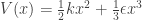Now imagine that in addition to the harmonic part of the potential, we also have a small additional component such that , so that the potential now looks like so:

The equation of motion is now nonlinear:

where and are constants. It is easy to see that if the amplitude of oscillations is small enough, there will be very little difference between this case and the case of the perfectly harmonic potential.

However, if the amplitude of the oscillations gets a little larger, there will clearly be deviations from the pure sinusoid. So then what does the position of the oscillator look like as a function of time? Perhaps not too surprisingly, considering the title, is that not only are there oscillations at , but there is also an introduction of a harmonic component with .

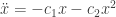
While the differential equation can’t be solved exactly without resorting to numerical methods, that the harmonic component is introduced can be seen within the framework of perturbation theory. In this context, all we need to do is plug the solution to the simple harmonic oscillator, into the nonlinear equation above. If we do this, the last term becomes:

,

showing that we get oscillatory components at twice the natural frequency. Although this explanation is a little crude — one can already start to see why nonlinearity often leads to higher frequency harmonics.

With respect to optical second harmonic generation, there is also one important ingredient that should not be overlooked in this simplified model. This is the fact that frequency doubling is possible only when there is an  component in the potential. This means that the potential needs to be inversion asymmetric. Indeed, second harmonic generation is only possible in inversion asymmetric materials (which is why ferroelectric materials are often used to produce second harmonic optical signals).

Because of its conceptual simplicity, it is often helpful to think about physical problems in terms of the classical harmonic oscillator. It would be interesting to count how many Nobel Prizes have been given out for problems that have been reduced to some variant of the harmonic oscillator!

Angular Momentum and Harmonic Oscillators

There are many analogies that can be drawn between spin angular momentum and orbital angular momentum. This is because they obey identical commutation relations:

    &     .

One can circularly permute the indices to obtain the other commutation relations. However, there is one crucial difference between the orbital and spin angular momenta: components of the orbital angular momentum cannot take half-integer values, whereas this is permitted for spin angular momentum.

The forbidden half-integer quantization stems from the fact that orbital angular momentum can be expressed in terms of the position and momentum operators:

.

While in most textbooks the integer quantization of the orbital angular momentum is shown by appealing to the Schrodinger equation, Schwinger demonstrated that by mapping the angular momentum problem to that of two uncoupled harmonic oscillators (pdf!), integer quantization easily follows.

I’m just going to show this for the -component of the angular momentum since the – and -components can easily be obtained by permuting indices. can be written as:

As Schwinger often did effectively, he made a canonical transformation to a different basis and wrote:

,

where is just some variable with units of length. Now, since the transformation is canonical, these new operators satisfy the same commutation relations, i.e. , and so forth.

If we now write in terms of the new operators, we find something rather amusing:

.

With the substitution , can be written as so:

.

Each of the two terms in brackets can be identified as Hamiltonians for harmonic oscillators with angular frequency, , equal to one. The eigenvalues of the harmonic oscillator problem can therefore be used to obtain the eigenvalues of the -component of the orbital angular momentum:

,

where denotes the Hamiltonian operator of the oscillator. Since the can only take integer values in the harmonic oscillator problem, integer quantization of Cartesian components of the angular momentum also naturally follows.

How do we interpret all of this? Let’s imagine that we have spins pointing up and spins pointing down. Now consider the angular momentum raising and lowering operators. The angular momentum raising operator in this example, , corresponds to flipping a spin of angular momentum, from down to up. The corresponds to the creation (annihilation) operator for oscillator 1 (2). The change in angular momentum is therefore . It is this constraint, that we cannot “destroy” these spins, but only flip them, that results in the integer quantization of orbital angular momentum.

I find this solution to the forbidden half-integer problem much more illuminating than with the use of the Schrodinger equation and spherical harmonics. The analogy between the uncoupled oscillators and angular momentum is very rich and actually extends much further than this simple example. It has even been used in papers on supersymmetry (which, needless to say, extends far beyond my realm of knowledge).

Phase Difference after Resonance

If you take the keys out of your pocket and swing them very slowly back and forth from your key chain, emulating a driven pendulum, you’ll notice that the keys swing back and forth in phase with your hand. Now, if you slowly start to speed up the swinging, you’ll notice that eventually you’ll hit a resonance frequency, where the keys will swing back and forth with a much greater amplitude.

If you keep slowly increasing the frequency of your swing beyond the resonance frequency, you’ll see that the keys don’t swing up as high. Also, you will notice that the keys now seem to be swaying out of phase with your hand (i.e. your hand is going in one direction while the keys are moving in the opposite direction!). This change of phase by 180 degrees between the driving force and the position of the oscillator is a ubiquitous feature of damped harmonic motion at frequencies higher than the resonance frequency. Why does this happen?

To understand this phenomenon, it helps to write down the equation for damped, driven harmonic motion. This could be describing a mass on a spring, a pendulum, a resistor-inductor-capacitor circuit, or something more exotic. Anyway, the relevant equation looks like this:

Let’s describe in words what each of the terms means. The first term describes the resistance to change or inertia of the system. The second term represents the damping of the system, which is usually quite small. The third term gives us the pullback or restoring force, while the last term on the right-hand side represents the external driving force.

With this nomenclature in place, let’s move on to what actually causes the phase change. First, we have to turn this differential equation into an algebraic equation by doing a Fourier transform (or similarly assuming a sinusoidal dependence of everything). This leaves us with the following equation:

Now we can more easily visualize what is going on if we concentrate on the left-hand side of the equation. Note that this equation can also suggestively be written as:

For small driving frequencies, , we see that the restoring term is the largest. The phase difference can then be represented graphically on an Argand diagram, where we can draw the following picture:

Restoring term dominates for low frequency oscillations

Therefore, the restoring force dominates the other two terms and the phase difference between the external force and the position of the oscillator is small (approximately zero).

At resonance, however, the driving frequency is the same as the natural frequency. This causes the restoring and inertial terms to cancel each other out perfectly, resulting in an Argand diagram like this:

 

Equal contribution from the restoring and inertial terms

After adding the vectors, this results in the arrow pointing upward, which is equivalent to saying that there is a 90 degree phase difference between the driving force and position of the oscillator.

You can probably see where this is going now, but let’s just keep going for the sake of completeness. For the case where the driving frequency exceeds the natural frequency (or resonant frequency), , we see that the inertial term starts to dominate, resulting in a phase shift of 180 degrees. This is again can be represented with an Argand diagram, as seen below:

Inertial term dominates for high frequency oscillations

This expresses the fact that the inertia can no longer “keep up” with the driving force and it therefore begins to lag behind. If the mass in a mass-spring system were to be reduced, the oscillator would be able to keep up with the driver up to a higher frequency. In summary, the phase difference can be plotted against the driving frequency to yield:

This phase change can be observed in so many contexts that it would be near impossible to list them all. In condensed matter physics, for instance, when sweeping the incident frequency of light in a reflectivity experiment of a semiconductor, a phase difference arises between the photon and the phonon above the phonon frequency. The problem that actually brought me to this analysis was the ported speaker, where above the resonant frequency of the speaker cone, the air from the port and the pressure wave generated from the speaker go 180 degrees out of phase.